Joining and dissolving in PostgreSQL: Castellon’s population by regions

Exercise 2: JOINS

Exercise 2 A

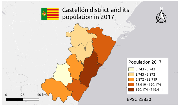
Complete the information from the MUNICIPIOS.shp layer with the information contained in the tables COMARAS_CASTELLON and POBLACION_CASTELLON. Represent the regions from the province of Castellon and the population grouped in 5 categories according to the natural Jenk breaks.

Layers to use:

• MUNICIPIOS.shp (municipalities)
• COMARCAS_CASTELLON (regions)
• POBLACION_CASTELLON (population)

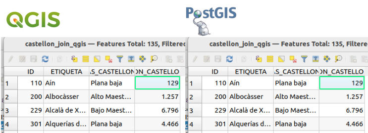
PostGIS is the CLI approach, while QGIS is the GUI approach.

PostGIs

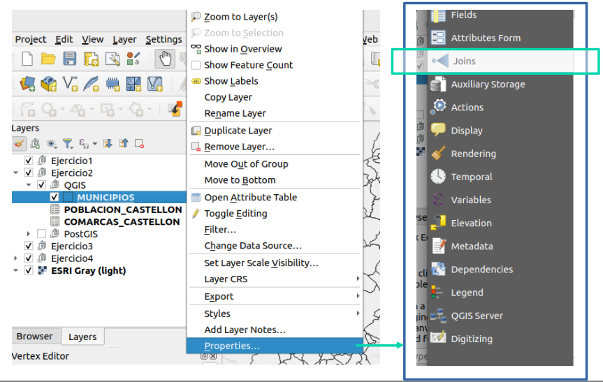
Joins: Adding regions data using joins

CREATE TABLE join_castellon_comarca_pop AS
SELECT 
    m."CODIGO_INE",
    m."ETIQUETA" as poblacion,
    c."Comarca" as comarca,
    p."2017_1" as pop_2017,
    m.geom as geom,
    st_centroid(m.geom) as pt_geom
FROM 
    municipios AS m
LEFT JOIN
    comarcas_castellon AS c ON c."CODIGO_INE" = m."CODIGO_INE"::integer
LEFT JOIN 
    poblacion_castellon AS p ON p."INE" = m."CODIGO_INE"::integer;

Groupping: Summarising data by regions

CREATE TABLE castellon_comarcas_pop_2017 AS
SELECT
        st_union(a.geom) as geom,
        st_centroid(st_union(a.geom)) as pt_geom,
        sum(pop_2017) as pop_comarca,
        comarca
FROM join_castellon_comarca_pop  AS a
GROUP BY comarca;

QGIS

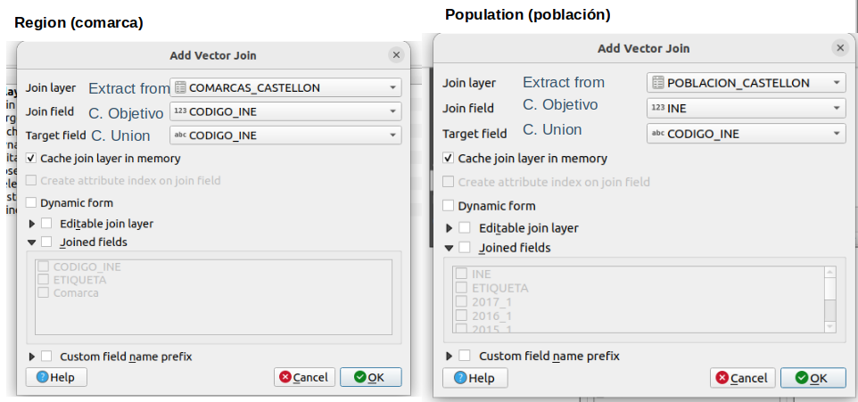
Joining data to the municipalities from regions

Uniting the municipalities geometry by region

Results

Municipalities choropleth map

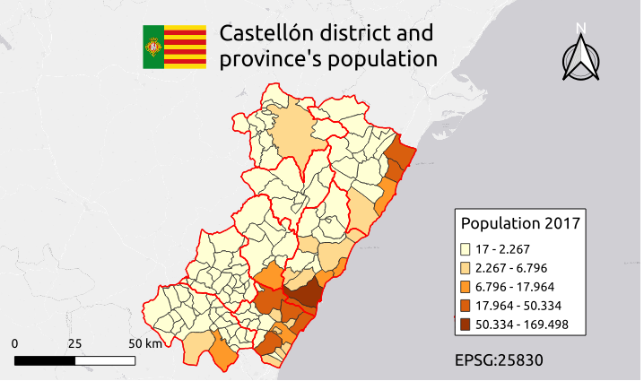
Region choropleth map

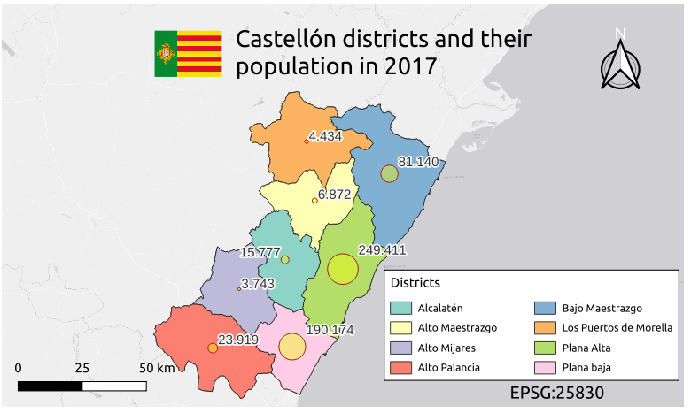
Region proportional map

Exercise 2 B

Obtén una capa llamada AVES.shp, a partir de los datos ornitológicos recogidos en el informe “general.csv”, que fueron obtenidos en el S.C. ETRS89 UTM 30N (EPSG25830) durante los trabajos de campo de octubre de 2013.

Descargar del IGN el BCN 200 de la comunidad de Madrid y utilizar la capa de núcleos de población BCN200_0501S_NUC_POB.shp. Las capacas facilitadas se encuentran en el S.C. ETRS89 EPGS 4258.

Obtener cual es el avistamiento más próximo a cada núcleo de población del ámbito de estudio.

Nota: Para realizar cálculos de distancia es importante que todas las capas se encuentran en un SIstema de Coordenadas Proyecto (UTM). Capas a utilizar:

• Ambiente_Estudio.shp
• BCN200_0501S_NUC_POB.shp
• general.csv

Importing the data using ogr2ogr. Unlike the QGIS workflow, PostGIS allows to have different SRID from different tables in the same schema.

PGCLIENTENCODING=LATIN1 ogr2ogr -f PostgreSQL PG:"host=localhost port=25432 user=docker password=docker dbname=gis schemas=tycgis" BCN200_0501S_NUC_POB.shp -nln nucleo_urbano -lco GEOMETRY_NAME=geom -nlt PROMOTE_TO_MULTI

PGCLIENTENCODING=LATIN1 ogr2ogr -f PostgreSQL PG:"host=localhost port=25432 user=docker password=docker dbname=gis schemas=tycgis" AMBITO_ESTUDIO_25830.shp -nln ambito_estudio -lco GEOMETRY_NAME=geom -nlt PROMOTE_TO_MULTI

--- Rename the General table to its lowercase option, so there is no need to use quotes to call the table.
ALTER TABLE "General"
RENAME TO general;
--- Create the table
CREATE TABLE general_postgis AS
SELECT 
    id,
    st_setsrid(
        st_makepoint("X_UTM","Y_UTM"), --- create Point
            25830) AS geom_postgis --- assign SRID
FROM general;

CREATE TABLE aves_closest_postgis AS    
WITH nucleo_urbano_25830 AS (
SELECT 
 nucleo_urbano.*,
 st_transform(nucleo_urbano.geom,
    st_srid(ambito_estudio.geom)) AS geom_25830 
FROM 
    nucleo_urbano,
    ambito_estudio
),---- table that includes the geometry reprojected at 25830
nucleo_ambito AS (
SELECT 
    DISTINCT ON (id) --- very important, otherwise, duplicates
    nucleo_urbano_25830.*
FROM 
    nucleo_urbano_25830,
    ambito_estudio
  WHERE st_intersects(nucleo_urbano_25830.geom_25830,
                    ambito_estudio.geom))
SELECT  
    nucleo_ambito.etiqueta AS nucleo,
    st_transform(aves.geom,4326)::geography
    <-> 
    st_transform(nucleo_ambito.geom_25830, 4326)::geography
    AS distance, --- <-> only works with 4326, it returns m
    aves.*
FROM nucleo_ambito
LEFT JOIN LATERAL
    (SELECT "N_comun",
                "Hora",
                "Fecha",
                aves.geom
     FROM 
        general_postgis AS aves
     ORDER BY
        aves.geom <-> nucleo_ambito.geom_25830
     LIMIT 1)   AS aves ON true;

For IMFE

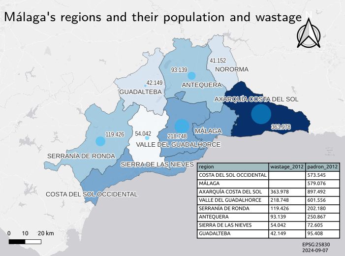
The provinces, NUTS 3, are obtained from Malaga Province Geoportal. Instead of the population, the amount of solid waste is chosen. As I was taught during my studies as laboratory technician, in the context of microbiology the population is determined by the amount of waste that is produced. Probably this is not applicable to a human urban context, since there may be influenced from other factors such as industries or other socioeconomic variables. The amount of waste is obtained through the Open Data Portal from Málaga

These are the layers:

• sitmap_municipios_view.shp (municipalities)
• sitmap_comarcas.shp (regions)
• resumen-anual-de-datos-residuos_v2.csv (waste)

Joins: Adding district data using joins

CREATE TABLE join_agp_comarca_waste AS
SELECT 
    m."codigo",
    m.nombre as municipality,
    m.padron as population,
    c.nombre as region,
    c.codigo as region_cod,
    w."RSU Toneladas Año" as waste_2012,
    m.geom as geom,
    st_centroid(m.geom) as pt_geom
FROM 
    agp_municipalities AS m
LEFT JOIN
    agp_comarcas AS c ON m.cod_comarc = c.codigo
LEFT JOIN 
    agp_waste AS w ON w."ID_Municipio"::integer = m."codigo"::integer;

Groupping: Summarising data

CREATE TABLE agp_comarcas_waste_2012 AS 
SELECT 
    region,
    st_union(geom) as geom,
    st_centroid(st_union(geom)) as pt_geom,
    SUM(waste_2012::float) AS waste_2012,
    SUM(population::float) AS padron_2012,
    region_cod::integer
FROM join_agp_comarca_waste
GROUP BY region_cod, region;

Results

Proportional map & Choropleth

There is a positive correlation between the wastage and the population. As waste increases, there is an increase in population. In fact, sorting the data by the waste or the population returned the same relative position, except for Sierra de las Nieves and Guadalteba.

An anomaly is the lack of data for two of the most populated regions, Málaga (the city center) and the “Costa del sol Occidental (the most touristic area) with known municipalities such as Marbella or Fuengirola. An unexpected finding was Axarquía as the region with most population, this could be explained by the misinterpretation of”padron” as population.

Overall, the wastage was a good proxy of population in relative terms.